Eulerian Video Magnification in real time in the browser

Some of the most interesting signals in a video are the ones we cannot see. The subtle flush of blood through a person’s face with every heartbeat, the near-imperceptible rise and fall of a sleeping baby’s chest, or the tiny vibration of a guitar string are all present in the pixels but far too small for the eye to register. Eulerian Video Magnification (EVM), introduced by Wu et al. at MIT CSAIL in 2012, is a technique for taking an ordinary video and amplifying exactly these changes, making the invisible visible.

This post describes an implementation I built of EVM. It starts with the core idea behind the algorithm, walks through the processing pipeline (color space, spatial pyramids, temporal filtering, and amplification), and explains how I restructured the classic offline method into a causal pipeline that runs frame-by-frame. Finally, it covers how to to run it live in the browser at real-time frame rates using a webcam, with no backend server involved.

EVM side-by-side

The core idea: an Eulerian point of view

There are two ways to think about motion in a video. The Lagrangian approach tracks features as they move through space. It estimates an optical-flow field, follows each particle, and exaggerates its trajectory. This is powerful but expensive and fragile: it needs accurate motion estimation, which is what breaks down for the tiny movements we care about.

EVM takes the Eulerian view, borrowed from fluid dynamics. Instead of tracking anything, we fix our gaze on each pixel and watch how its value changes over time. A pixel sitting on the edge of someone’s wrist will brighten and darken slightly as a vein pulses beneath it. We never ask “where did this edge go?”, we only ask “how did the intensity at this fixed location vary?”, then amplify that variation.

The insight that makes this equivalent to motion magnification is a first-order Taylor expansion. If an image $I(x, t)$ undergoes a small translation $\delta(t)$, then

$$I(x, t) = f\big(x + \delta(t)\big) \approx f(x) + \delta(t)\,\frac{\partial f(x)}{\partial x}.$$

The temporal variation at a fixed pixel is approximately $\delta(t)$ scaled by the local spatial gradient. If we isolate a band of temporal frequencies (say, the 1 Hz of a resting heartbeat) and add an amplified copy $\alpha$ of it back to the frame, the result is approximately

$$f(x) + (1 + \alpha)\,\delta(t)\,\frac{\partial f(x)}{\partial x} \approx f\big(x + (1 + \alpha)\,\delta(t)\big),$$

which is exactly the original motion, magnified by a factor of $(1 + \alpha)$. The beauty of it is that we get motion magnification without ever computing motion.

The processing pipeline

Every frame flows through five stages. I’ll use the Python core as the reference.

1. Separate color from brightness

The first step converts each frame from RGB into YIQ color space, which splits a pixel into a luminance channel (Y) and two chrominance channels (I and Q):

_RGB2YIQ = np.array([
    [0.299,  0.587,  0.114],
    [0.596, -0.274, -0.322],
    [0.211, -0.523,  0.312],
], dtype=np.float64)

This matters because motion and color changes live in different channels. Small movements mostly show up in luminance, while a heartbeat’s blood-flow signal is a subtle color shift. Working in YIQ lets us amplify luminance and chrominance by different amounts, which is essential for keeping color noise under control later.

2. Build a Laplacian pyramid

Motion in a video happens at many spatial scales — a big nod of the head versus the flicker of an eyelid — so it makes sense to process each scale independently. For that we decompose every frame into a Laplacian pyramid.

The construction is the classic one: repeatedly blur-and-downsample the image with cv2.pyrDown() to form a Gaussian pyramid, then take the difference between each level and the upsampled version of the level below it.

def build_laplacian_pyramid(frame, levels):
    gaussian = frame
    pyramid = []
    for _ in range(levels):
        down = cv2.pyrDown(gaussian)
        up = cv2.pyrUp(down, dstsize=(gaussian.shape[1], gaussian.shape[0]))
        pyramid.append(gaussian - up)   # band-pass detail at this scale
        gaussian = down
    pyramid.append(gaussian)            # low-frequency residual
    return pyramid

Each level holds the spatial detail in one frequency band, and the final level is the coarse residual. The pyramid depth is chosen automatically from the frame size, roughly $\lfloor \log_2(\min(h, w)) \rfloor - 2$, and capped at a few levels so it stays fast.

3. Filter in time

This is the heart of EVM. For each pyramid level, we run a temporal band-pass filter across frames to keep only the changes happening within the frequency band of interest. For a pulse, that is roughly $0.75$–$3\,\text{Hz}$, i.e. 45–180 beats per minute.

The original paper does this offline, running an ideal band-pass filter over the whole video at once with an FFT. That is not an option for a live stream, where future frames simply don’t exist yet. Instead we use a causal recursive filter built from two first-order Butterworth low-pass filters — one at the low cutoff and one at the high cutoff. The band-pass output is their difference.

wl = np.clip(fl / (fps / 2.0), 0.01, 0.99)
wh = np.clip(fh / (fps / 2.0), 0.01, 0.99)
self.low_b,  self.low_a  = butter(1, wl, btype="low")
self.high_b, self.high_a = butter(1, wh, btype="low")

Each incoming frame updates the filter state using only the current and previous frame, so the whole thing runs in constant memory and never looks ahead:

self.lowpass1[lvl] = (-self.high_a[1] * self.lowpass1[lvl]
                      + self.high_b[0] * pyr[lvl]
                      + self.high_b[1] * self.pyr_prev[lvl]) / self.high_a[0]
self.lowpass2[lvl] = (-self.low_a[1] * self.lowpass2[lvl]
                      + self.low_b[0] * pyr[lvl]
                      + self.low_b[1] * self.pyr_prev[lvl]) / self.low_a[0]
filtered[lvl] = self.lowpass1[lvl] - self.lowpass2[lvl]

4. Amplify, with a wavelength-aware gain

It’s tempting to just multiply the filtered signal by a single large $\alpha$, but that also amplifies noise as much as signal, especially at the finest scales. EVM instead ties the gain to the spatial wavelength $\lambda$ of each pyramid level, so that coarse levels (large, reliable motions) get amplified more and fine levels (where noise dominates) get held back.

$$\alpha_\text{level} = \frac{\lambda}{8\,\delta} - 1, \qquad \delta = \frac{\lambda_c}{8\,(1 + \alpha)}.$$

Here $\lambda_c$ is a cutoff wavelength: detail finer than $\lambda_c$ is progressively attenuated. In practice I also zero out the very finest and the residual levels outright, clamp the per-level gain to the user’s $\alpha$, and scale the chrominance channels by a small chrom_attenuation factor (around $0.1$) to suppress color fringing while still letting the blood-flow tint through.

5. Reconstruct and blend

Finally I collapse the amplified pyramid back into a full-resolution image and add it to the original frame. The sum is clipped to a valid range and converted back to RGB.

motion = reconstruct_from_laplacian(filtered)
output = np.clip(frame + motion, 0.0, 1.0)

That additive blend is the whole trick from the Taylor expansion earlier: adding back a scaled copy of the temporal variation is equivalent to magnifying the underlying motion.

Detecting a heartbeat

Since the pipeline already isolates the pulse band, extracting an actual beats-per-minute reading is a natural extension. The flow is:

Find a face. On the Python side I use an OpenCV Haar cascade; in the browser I try the native FaceDetector API and fall back to a simple skin-color heuristic when it isn’t available.
Focus on the forehead. I crop the upper-center third of the detected face, where skin is exposed, and cache the region so a momentarily missed detection doesn’t drop the signal.
Turn color into a pulse. The Python estimator averages the green channel over the forehead across a rolling window, band-passes it, and takes an FFT; the peak frequency in the $0.75$–$3\,\text{Hz}$ range gives the heart rate. The browser version uses the more robust CHROM method (de Haan & Jeanne, 2013), which combines the normalized R, G and B channels into a single chrominance pulse signal before running a DFT. It also carries a confidence score and smooths the estimate so the displayed number doesn’t jitter.

Heartbeat detection

Running it live in the browser

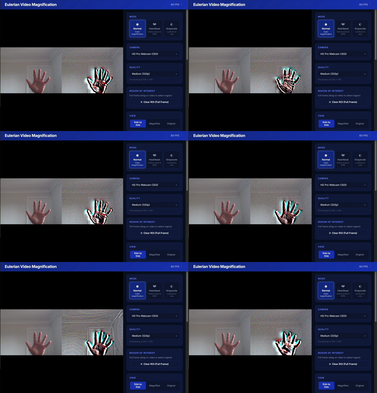
The browser client works with no backend and amplifies motion in real time. The entire EVM pipeline runs client-side in JavaScript.

The capture side uses getUserMedia:

const stream = await navigator.mediaDevices.getUserMedia({
    video: { width: { ideal: 640 }, height: { ideal: 480 }, frameRate: { ideal: 30 } },
    audio: false,
});
video.srcObject = stream;

Each animation frame draws the webcam into an off-screen canvas, pulls the pixels out with getImageData, feeds them through a LiveMagnifier instance, and writes the result back out:

function processFrame() {
    srcCtx.drawImage(video, 0, 0, processingWidth, processingHeight);
    const frame = srcCtx.getImageData(0, 0, processingWidth, processingHeight);
    const magnified = magnifier.process(frame);   // full EVM in JS
    outCtx.putImageData(magnified, 0, 0);
    composeDisplay();                              // side-by-side / single view
    requestAnimationFrame(processFrame);
}

Parameters and presets

EVM is sensitive to its parameters, and the “right” values depend entirely on what you’re trying to reveal. The main parameters are:

Parameter	Role
`alpha`	Overall amplification factor — how much to exaggerate
`lambda_c`	Spatial cutoff wavelength; finer detail is attenuated
`fl`, `fh`	Lower and upper bounds of the temporal band-pass
`chrom_attenuation`	How much to scale color vs. brightness
`filter_type`	Causal Butterworth band-pass, or the cheaper IIR pair

To make it approachable I wired up a few presets:

Face pulse — a narrow band around 1 Hz with modest gain, to reveal blood flow.
Breathing — a very low band ($0.1$–$0.5\,\text{Hz}$) to exaggerate slow chest movement.
Vibration — a high band with strong gain, for things like a plucked string or a running motor.

Closing thoughts

What I find satisfying about EVM is how much it gets from a simple change of perspective. By refusing to track motion and instead watching fixed pixels over time, it turns an intractable optical-flow problem into a stack of band-pass filters. Reworking the classic offline algorithm into a causal, per-frame pipeline was the key step that let it run live, and pushing that pipeline entirely into the browser meant the demo needs nothing more than a webcam and a tab.

The full source, including the browser demo and the Python server, is on GitHub.